2 直線を表すグラフ

直線とグラフ

• 座標上に直線を描画するには x軸、y軸の値（x, y）をいくつか（最低2組）決めて結ぶ

• x = [1, 2, 3, 4, 6]

• y = [1, 2, 3, 4, 5]

• (x, y)値をプロットし各プロットを結ぶと y = x という式で示される直線ができる

Matplotlib でグラフを描く

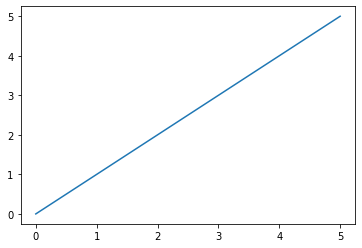
y = x のグラフをプログラミングする

• x の値は 0..5

• Matplotlib を使って描く

• %matplotlib inline … セル直下にグラフを表示するための jupyter notebook の命令

%matplotlib inline
import matplotlib.pyplot as plt # Matplotlib.Pyplotモジュール に plt という名前を付けて読み込む

x = [0, 1, 2, 3, 4, 5]    # x　座標
y = x                     # y　座標

plt.plot(x, y)            # 直線を描画
plt.show()                # 描画

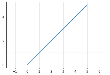
縦と橫の目盛りを描画する

x = [0, 1, 2, 3, 4, 5]     # x 座標
y = x                      # y 座標

plt.plot(x, y)             # 直線を描画
plt.grid(color='0.8')      # グリッドを薄グレーで描画する
plt.show()                 # 描画

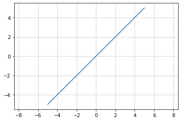
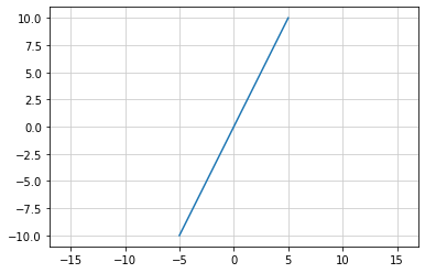
楯と橫の目盛りを揃えて描画する

x = [-5, -4, -3, -2, -1, 0, 1, 2, 3, 4, 5]     # x 座標
y = x                      # y 座標

plt.plot(x, y)             # 直線を描画
plt.axis('equal')          # 縦横の目盛りの大きさを揃える
plt.grid(color='0.8')      # グリッドを薄グレーで描画する
plt.show()                 # 描画

比例の式

• y = x

• y は x と等しく変化する

• y = nx

• y は x の n倍 に比例して変化する

• a は比例定数

y = x … y と x は比例関係にあり、その比例定数は 1 である

y = nx … y と x は比例関係にあり、その比例定数は n である

比例定数は n ≠ 0

関数とグラフ

• y = nx (n ≠ 0) … y は x の関数である

∵ x の値が1つに決まれば y の値も1つに決まる

y = x のグラフ

%matplotlib inline
import matplotlib.pyplot as plt

def func_1(x):
    return x                   # y = x

x = []
y = []
for i in range(-5, 6):         # i が －5 から 5 の間
    x.append(i)                 # x に i を追加
    y.append(func_1(i))          # func_1() の結果を y に追加

plt.plot(x, y)
plt.axis('equal')
plt.grid(color = '0.8')
plt.show()

y = 2x のグラフ

def func_2(x):
    return 2 * x                   # y = x

x = []
y = []
for i in range(-5, 6):         # i が －5 から 5 の間
    x.append(i)                 # x に i を追加
    y.append(func_2(i))          # func_1() の結果を y に追加

plt.plot(x, y)
plt.axis('equal')
plt.grid(color = '0.8')
plt.show()

y = nx (n=0) のグラフ

def func_3(x):
    return n * x                   # y = x

n = input('n = ')                   # 定数 n を入力（ n は 整数か小数）
n = float(n)                        # n を実数化
x = []
y = []
for i in range(-5, 6):            # i が －5 から 5 の間
    x.append(i)                    # x に i を追加
    y.append(func_3(i))            # func_1() の結果を y に追加

plt.plot(x, y)
plt.axis('equal')
plt.grid(color = '0.8')
plt.show()

n = 0

直線の傾きを決めるもの

• y = ax … a が変わると傾きが変わる

• a = y/x … a は変化の割合で y/x で求められる

%matplotlib inline
import matplotlib.pyplot as plt

def func_3(x):
    return 2 / 3 * x

x = []
y = []

for i in range(-5, 6):
    x.append(i)
    y.append(func_3(i))

plt.plot(x, y)
plt.axis('equal')
plt.grid(color = '0.8')
plt.show()

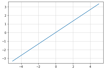
傾きが n / m の直線を描画する

def func_3(x):
    return n / m * x

m = input('m = ')
n = input('n = ')
m = float(m)
n = float(n)

x = []
y = []

for i in range(-5, 6):
    x.append(i)
    y.append(func_3(i))

plt.plot(x, y)
plt.axis('equal')
plt.grid(color = '0.8')
plt.show()

m = -5
n = 2

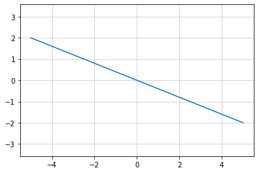
座標軸に平行な直線

① y = ax で直線が描ける

② a は直線の傾きを示す

③ a > 0 の時には右上がり、a < 0 の時には右下がりの直線になる

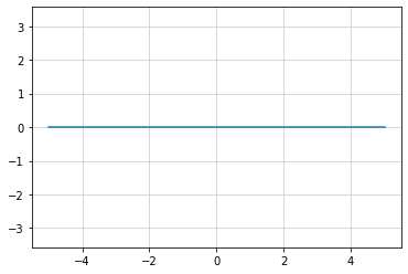
- a = 0 の時にはどのようになるか？

def func_5(x):
    return n / m * x

m = input('m = ')
n = input('n = ')
m = float(m)
n = float(n)

x = []
y = []

for i in range(-5, 6):
    x.append(i)
    y.append(func_5(i))

plt.plot(x, y)
plt.axis('equal')
plt.grid(color = '0.8')
plt.show()

m = 1
n = 0

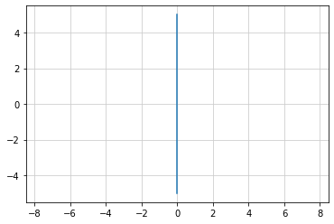
x = 0 の時にはどのようになるか？

• y 軸に平行な直線となる

• この式は関数では無い

x = [0, 0]
y = [-5, 5]

plt.plot(x, y)
plt.axis('equal')
plt.grid(color = '0.8')
plt.show()

直線の位置を決めるもの

• y = ax … 定数a と 変数x との乗算が 変数y の値となる

• x軸 と y軸 の二次元グラフで表すと 原点（0, 0）を通る傾きが a の直線となる

• y = ax + b ….原点以外を通る直線の式

• b は x = 0 の時の y の値、y軸の切片となる

y = 2x と y = 2x + 3 のグラフを同じプロットに描画する

%matplotlib inline
import matplotlib.pyplot as plt

def func_b0(x):
    return 2 * x

def func_b5(x):
    return 2 * x + 5

x = []
y1 = []
y2 = []

for i in range(-5,6):
    x.append(i)
    y1.append(func_b0(i))
    y2.append(func_b5(i))

plt.plot(x, y1)
plt.plot(x, y2)
plt.axis('equal')
plt.grid(color = '0.8')
plt.show()

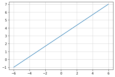
傾きが n/m、切片が b の直線を描く

def func_s(x):
    return (n / m) * x + b

b = input('b = ')
m = input('m = ')
n = input('n = ')

print('y = (n / m) * x + b ')
b = float(b)
m = float(m)
n = float(n)

x = []
y = []

for i in range(-6,7):
    x.append(i)
    y.append(func_s(i))

plt.plot(x, y)
plt.axis('equal')
plt.grid(color = '0.8')
plt.show()

b = 3
m = 3
n = 2
y = (n / m) * x + b

直線をあらわす式

• 直線の傾きを a 、切片を b とする平面上の直線は y = ax + b であらわされる

• 切片は x = 0 の時の y の値で、y軸の原点からの距離

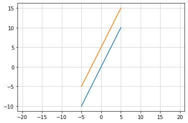
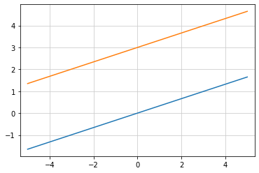
平行線（1）

%matplotlib inline
import matplotlib.pyplot as plt

import numpy as np

# 原点を通る直線
def func_dline(x):
    return 2 * x

# 切片 -10 の直線
def func_line(x):
    return 2 * x - 10

# 1本目の直線
x1 = np.arange(-1.5, 2)
y1 = func_dline(x1)
plt.plot(x1, y1)

# 2本目の直線
x2 = np.arange(-1.5, 6)
y2 = func_line(x2)
plt.plot(x2, y2)

# 表示
plt.grid(color = '0.8')
plt.axis('equal')
plt.show()

平行線（2）

%matplotlib inline
import matplotlib.pyplot as plt

import numpy as np

# 原点を通る直線
def func_zline(x):
    return a * x

# 切片 -10 の直線
def func_line(x):
    return a * x + b

a = float(input('直線の傾き =  '))
b = float(input('切片 = '))
m = float(input('x の範囲 ='))

# 1本目の直線
x1 = np.arange(-m, m+1)
y1 = func_zline(x1)
plt.plot(x1, y1)

# 2本目の直線
x2 = np.arange(-m, m+1)
y2 = func_line(x2)
plt.plot(x2, y2)

# 表示
plt.grid(color = '0.8')
plt.axis('equal')
plt.show()

# NumPy の配列を使うとプログラムが簡単になる

直線の傾き =  0.33
切片 = 3
x の範囲 =5

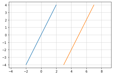
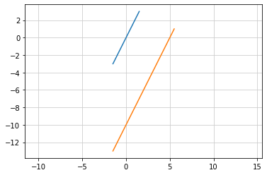
横方向に並んだ2つの直線（1）

# 原点を通る直線
def func_az(x):
    return 2 * x

# x 軸方向に平行移動した直線
def func_a(x):
    return 2 * (x - 4.5)

# 原点を通る直線
x1 = np.arange(-2, 2)
y1 = func_az(x1)
plt.plot(x1, y1)

# x 軸に平行移動した直線
x2 = x1 + 4.5
y2 = func_a(x2)
plt.plot(x2, y2)

# 表示
plt.grid(color = '0.8')
plt.show()

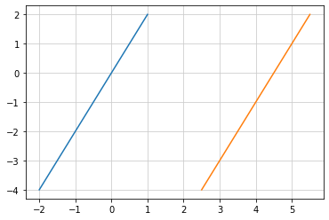
横方向に並んだ2つの直線（2）

# 原点を通る直線
def func_az(x):
    return a * x

# x 軸方向に平行移動した直線
def func_a(x):
    return a * (x - c)

a = float(input('直線の傾き = '))
c = float(input('平行移動した直線が x軸 と交わる x値 = '))
m = float(input('直線の始まりの x値 = '))
n = float(input('直線の終わりの x値 = '))

# 原点を通る直線
x1 = np.arange(m, n)
y1 = func_az(x1)
plt.plot(x1, y1)

# x 軸に平行移動した直線
x2 = x1 + c
y2 = func_a(x2)
plt.plot(x2, y2)

# 表示
plt.grid(color = '0.8')
plt.axis('equal')
plt.show()

直線の傾き = 2
平行移動した直線が x軸 と交わる x値 = 5
直線の始まりの x値 = -2
直線の終わりの x値 = 3